If the filter input signal consists of a sine wave, the dynamic range of the filter depends on the frequency of this signal as follows.
DR(ω) = 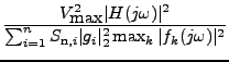 . .
|
(28) |
plot: dr;
Mainly to investigate the results of dynamic-range optimization with a weighting function or using a single frequency, the plot specifications drfact, drscfact and dropfact were incorporated. drfact specifies a plot of the normalized dynamic range as a function of frequency. drscfact specifies for each frequency the normalized dynamic range that can be reached if the filter is scaled for that specific frequency. dropfact specifies the normalized dynamic range that can be reached if the filter is optimized by do for that specific frequency. This means that the dynamic range factors as plotted by drscfact and dropfact can never be reached by one and the same filter at all frequencies, but usually at only one frequency.
The definitions of these factors are:
drfact = 
|
(29) |
drscfact = 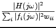
|
(30) |
dropfact = 
|
(31) |
These plotting specifications yield illustrative pictures for a filter that is optimized at one frequency.