Consider the following input file.
butterworth(3);
ctot = 3e-12;
umax = 1;
freq=lin(0,5,100);
output: dr;
plot: magn(f);
which specifies a third-order Butterworth filter. The output file is
Output noise level: 1.174904e-04 V.
Scaling is L-infinity.
Maximum output level: 6.314818e-01 V.
Dynamic range: 5.374751e+03 (74.61 dB).
and the result of the plot command is in Figure 12.
 |
To equalize the integrator output signal levels, use
transform: scale;Adding this somewhere between the butterworth(3); command and the output: dr; command results in the following output file
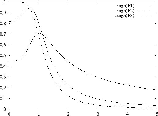
Output noise level: 1.370834e-04 V.
Scaling is L-infinity.
Maximum output level: 1.000000e+00 V.
Dynamic range: 7.294827e+03 (77.26 dB).
and the internal transfer function plot of Figure 13. All internal transfer functions peak at a value of 1, and the dynamic range has increased by 2.65dB.
This form of scaling is appropriate if the input signal is a sinusoid with unknown frequency. It is known by the name L∞ scaling. This is the default type of scaling in FA.
In case of L∞ scaling, the program has to find the tops of the internal transfer functions. It may find a local peak. FA does an initial grid search to prevent this. It compresses the frequency range from zero to infinity into the interval [0, 1] and divides this into a number of steps. It evaluates the transfer functions at each step to find an initial estimate for the global maximum. The default number of steps is 50. The number of steps can be changed with the command
scale_grid = <int>
If the input signal is not a sinusoid with unknown frequency, but a wide-band signal as explained in Section 10.2, equalizing the peaks of the internal transfer functions will not optimize the dynamic range. In this case the integrals of the squared magnitudes of the transfer functions must be equalized. This is a form of scaling known as L2 scaling. FA will use this type of scaling if the scale2 flag is set, as in set: scale2;.
As an example, this input file
butterworth(3);
ctot = 3e-12;
umax = 1;
freq=lin(0,5,100);
set: scale2;
output: dr;
transform: scale;
output: dr;
plot: magn(f);
produces the following output
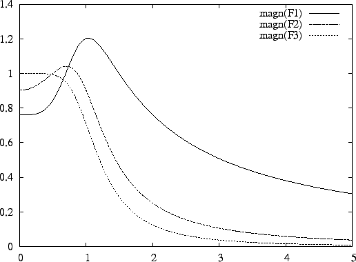
Output noise level: 1.174904e-04 V.
Scaling is L2.
Maximum output level: 4.472136e-01 V.
Dynamic range: 3.806383e+03 (71.61 dB).


Output noise level: 1.559230e-04 V.
Scaling is L2.
Maximum output level: 1.000000e-00 V.
Dynamic range: 6.413422e+03 (76.14 dB).
and the plot of Figure 14. This plot shows that the scaling operation did not equalize the peaks of the transfer functions, but the integrals of the squared magnitudes of the transfer functions. The scaling operation improved the dynamic range by 4.53dB.
The spectrum of the input signal may not be flat. For example, let the input spectral density be given by the formula
so that most of the spectral energy is present in the band from 0 to ωi . In FA, the variable si represents this input spectrum, and fr represents frequency. To make the spectrum frequency dependent, specify si as a function of fr. A specification of the spectrum (27) with ωi = 0.5 rad/s could besi = 1/((fr/0.5)^2+1);Additionally, FA needs to be instructed to determine internal signal levels by numeric integration and not by solving a set of equations, as follows.
set: num;An example FA input file is
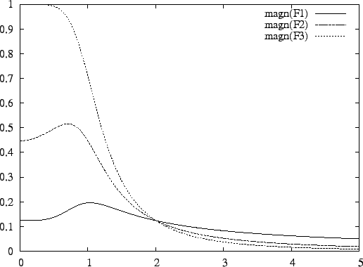
butterworth(3);
ctot = 3e-12;
umax = 1;
freq=lin(0,5,100);
set: num scale2;
si = 1/((fr/0.5)^2+1);
output: dr;
transform: scale;
output: dr;
plot: magn(f);
which gives the result
Output noise level: 1.174904e-04 V. Scaling is L2. Maximum output level: 7.608857e-01 V. Dynamic range: 6.476151e+03 (76.23 dB). Output noise level: 1.288175e-04 V. Scaling is L2. Maximum output level: 1.000000e+00 V. Dynamic range: 7.762919e+03 (77.80 dB).and the internal transfer function plot of Figure 15.
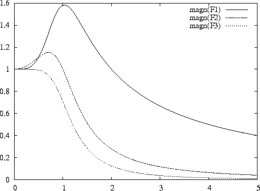
Finally, consider the example where there is a strong blocker at 2rad/s.
To specify this, set the sfr and the scale2 flags, and
assign the frequency of the blocker to the variable fr, as follows.
butterworth(3);
ctot = 3e-12;
umax = 1;
freq=lin(0,5,100);
set: sfr scale2;
fr = 2;
output: dr;
transform: scale;
output: dr;
plot: magn(f);
The FA output is
Output noise level: 1.174904e-04 V. Scaling is L2. Maximum output level: 1.240347e-01 V. Dynamic range: 1.055701e+03 (60.47 dB). Output noise level: 3.486558e-04 V. Scaling is L2. Maximum output level: 1.000000e+00 V. Dynamic range: 2.868159e+03 (69.15 dB).and the internal transfer function plot of Figure 16.