State-Space Representation

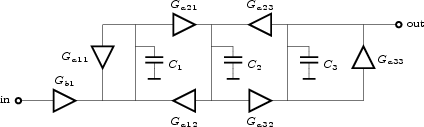
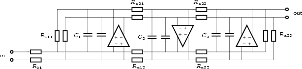
Figure 3 shows an active realization of a third-order ladder

Figure 3: An active lowpass ladder filter.

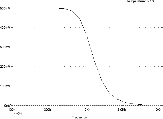
filter. The filter consists of a network of transadmittance stages and capacitors. With C₁ = C₂ = C₃ = 100pF , G_b1 = 6.283⋅10^-7 A/V, G_a11 = G_a33 = - 6.283⋅10^-7 A/V, G_a21 = G_a32 = - 4.443⋅10^-7 A/V and G_a12 = G_a23 = 4.443⋅10^-7 A/V the filter is a Butterworth type lowpass filter with a cutoff frequency of 1kHz. Figure 4 shows the results of a SPICE transfer-function analysis of the circuit.

Figure 4: The transfer function of the filter of Figure 3.

The capacitors in the filter act as integrators, and the voltages on the capacitors are the output voltages of these integrators. These voltages form the state variables x_i of the filter. Let x_i designate the voltage over C_i . It is not difficult to derive the network equations in terms of the state variables:

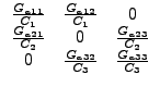
sC₁x₁ = G_a11x₁ + G_a21x₂ + G_b1V_in (1)

sC₂x₂ = G_a21x₁ + G_a23x₃ (2)

sC₃x₃ = G_a32x₂ + G_a33x₃ (3)

V_out = x₃, (4)

where V_in and V_out are the input and output voltages of the filter. Define the state vector X as

X = $$\left(\vphantom{ \begin{array}{c} x_1 \\ x_2 \\ x_3 \end{array} }\right.$$$$\begin{array}{c} x_1 \\ x_2 \\ x_3 \end{array}$$$$\left.\vphantom{ \begin{array}{c} x_1 \\ x_2 \\ x_3 \end{array} }\right)$$

then the network equations become

sX = AX + BV_in (5)

V_out = CX + DV_in (6)

with

A	=	$$\left(\vphantom{ \renewedcommand{arraystretch}{1} \begin{array}... ...{C_2} \\ 0 & \frac{G_{a32}}{C_3} & \frac{G_{a33}}{C_3} \end{array} }\right.$$$$\begin{array}{ccc} \frac{G_{a11}}{C_1} & \frac{G_{a12}}{C_1} & 0... ...{G_{a23}}{C_2} \\ 0 & \frac{G_{a32}}{C_3} & \frac{G_{a33}}{C_3} \end{array}$$$$\left.\vphantom{ \renewedcommand{arraystretch}{1} \begin{array}... ...{C_2} \\ 0 & \frac{G_{a32}}{C_3} & \frac{G_{a33}}{C_3} \end{array} }\right)$$		B	=	$$\left(\vphantom{ \renewedcommand{arraystretch}{1} \begin{array}{c} \frac{G_{b1}}{C_1} \\ 0 \\ 0 \end{array} }\right.$$$$\begin{array}{c} \frac{G_{b1}}{C_1} \\ 0 \\ 0 \end{array}$$$$\left.\vphantom{ \renewedcommand{arraystretch}{1} \begin{array}{c} \frac{G_{b1}}{C_1} \\ 0 \\ 0 \end{array} }\right)$$
C	=	$$\left(\vphantom{ \renewedcommand{arraystretch}{1} \begin{array}{ccc} 0 & 0 & 1 \end{array} }\right.$$$$\begin{array}{ccc} 0 & 0 & 1 \end{array}$$$$\left.\vphantom{ \renewedcommand{arraystretch}{1} \begin{array}{ccc} 0 & 0 & 1 \end{array} }\right)$$		D	=	0.

(7)

or numerically:

A	=	$$\left(\vphantom{ \renewedcommand{arraystretch}{1} \begin{array}... ...& 4443 & 0 \\ -4443 & 0 & 4443 \\ 0 & -4443 & -6283 \end{array} }\right.$$$$\begin{array}{ccc} -6283 & 4443 & 0 \\ -4443 & 0 & 4443 \\ 0 & -4443 & -6283 \end{array}$$$$\left.\vphantom{ \renewedcommand{arraystretch}{1} \begin{array}... ...& 4443 & 0 \\ -4443 & 0 & 4443 \\ 0 & -4443 & -6283 \end{array} }\right)$$,		B	=	$$\left(\vphantom{ \renewedcommand{arraystretch}{1} \begin{array}{c} 6283 \\ 0 \\ 0 \end{array} }\right.$$$$\begin{array}{c} 6283 \\ 0 \\ 0 \end{array}$$$$\left.\vphantom{ \renewedcommand{arraystretch}{1} \begin{array}{c} 6283 \\ 0 \\ 0 \end{array} }\right)$$,
C	=	$$\left(\vphantom{ \renewedcommand{arraystretch}{1} \begin{array}{ccc} 0 & 0 & 1 \end{array} }\right.$$$$\begin{array}{ccc} 0 & 0 & 1 \end{array}$$$$\left.\vphantom{ \renewedcommand{arraystretch}{1} \begin{array}{ccc} 0 & 0 & 1 \end{array} }\right)$$		D	=	0.

(8)

Because these three matrices completely specify the structure of the filter, FA uses them for this purpose. A FA specification for this filter is

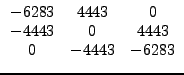
input :

order = 3;

A =
-6283   4443   0
-4443   0      4443
 0     -4443  -6283  ;

B =
6283
0
0 ;

C =
0 0 1 ;
;

The order of the filter must be specified first. Then the state matrices appear, in the order A , B , C , D . The input command as well as the matrix specifications each require a semicolon as termination character. The specification of D is optional. If there is no specification for D (as in this example) it receives a value of zero.

There are several ways to realize the filter network structure as described by matrices (8). One of these realizations is the filter of Figure 3. An alternative realization as an opamp-R-C filter is in Figure 5.

Figure 5: An opamp-R-C realization of the filter described by state matrices (8).

If the capacitor values are the same as in Figure 3, and the resistor values are the absolute values of the reciprocal values of the corresponding transadmittances, both examples will have the same state-space representation and transfer function.

Figure 6 shows a signal-flow diagram depicting the state-space model of the example filters of this section.

Figure 6: The signal flow graph for the filters of Figures 3 and 5.

If a user specifies a filter transfer function, FA will determine a network that realizes this transfer function and store the network in the state-space format. FA will show the state matrices if the user enters the command output: filter;. For instance, the input specification

chebyshev(4,0.1);
output: filter;

results in the following.

(4, 4)
  -6.377299e-01   4.650002e-01   0.000000e+00   0.000000e+00
  -4.650002e-01  -6.377299e-01   0.000000e+00   0.000000e+00
  -0.000000e+00  -1.184767e+00  -2.641564e-01   1.122610e+00
   0.000000e+00   0.000000e+00  -1.122610e+00  -2.641564e-01

B =
(4, 1)
  -1.339622e+00
   0.000000e+00
  -0.000000e+00
   0.000000e+00

C =
(1, 4)
   0.000000e+00   0.000000e+00   0.000000e+00   1.000000e+00

D = 0.000000e+00